Bound States as Symmetry Operators and E8

Previously, we saw that density operators generate symmetries in the set of quantum states and that these new symmetries gave non Hermitian quantum states. We then saw that bound states of Feynman diagrams can be represented by matrices of these non Hermitian quantum states. In this post, we use these matrices of non Hermitian quantum states, that is the bound states, to generate symmetries on all the quantum states, bound and free. This is necessary for the recursion that derives E8 as a consequence of treating bound states on an equal footing with free states.

The method of turning a matrix of density matrix states into a symmetry on matrices of density matrix states follows exactly our method of turning a density matrix into a symmetry of density matrices. Let U and V be arbitrary 3×3 matrices whose entries are complex multiples of density matrix states, and let S be an arbitrary 3×3 density matrix whose entries are complex multiples of density matrix states. Since S is a density matrix we have SS = S. The transformation on U is:

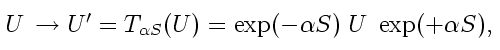
and the transformation on V is similar. As in the earlier density matrix case, this transformation preserves addition and multiplication, that is:

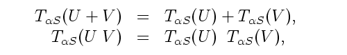
since the transformation is linear, that is, , and in the case of multiplication, the exponentials between the products cancel.

The definition of a density matrix are that the matrix (a) be idempotent (i.e. square to itself), and (b) have trace 1 (or be primitive in the mathematical language). Since multiplication is preserved, idempotency is satisfied. And since the trace function satisfies 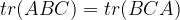, we can cancel the two exponentials against each other and the trace is preserved. Thus the above transformation does map density matrices (representing bound states) to density matrices (which we also interpret as representing bound states).

Bound States as Transformations of the Free States

So our bound states transform bound states to bound states — they are symmetries on the bound states. But our task is to build a tower of composite states that eventually ends when we have included all possible symmetries of the combined set of bound and composite states. To do that, we have to show that the bound states transform not only their own sort of bound states, but that they also transform the free states (both Hermitian and non Hermitian). To do this, we need to embed the free states in our bound state notation, and then show that the exponential map preserves them.

The 3×3 matrices in our example bound states have their nine entries labeled according to the free Hermitian density matrices that multiply to give them. The diagonal entries are products of identical free Hermitian density matrices, while the off diagonal entries are products of two distinct free Hermitian density matrices. Returning to the notation of the previous post, we will use X, Y, and Z for the diagonal free Hermitian density matrices, and the various products as the off diagonal terms. A general 3×3 matrix of complex multiples , of the products of these free density matrices is:

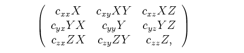
The nine complex numbers are to be arranged so that the matrix is a primitive idempotent, and so can be interpreted as a density matrix.

The pure Hermitian free density matrices are on the diagonal of the above matrix, so it is clear how they should be transformed. For example, to transform Y, we set all the to be zero except for . By setting the matrix this way, it will match the format of a bound state 3×3 density matrix: The matrix will be idempotent, and its trace will be 1.

In embedding the free non Hermitian density matrice into the bound state form, we may wish to be a little more careful because, for example, XY is not idempotent. But products of Hermitian primitive idempotents are real multiples of (generally non Hermitian) primitive idempotents. In this case, 2XY is a non Hermitian primitive idempotent, so we need to adjust the values of the by the real constant. In such a case, we set the constants to be zero except for the one we wish to transform, and that one we set to be 1, or 2, depending on how we wish to normalize the non Hermitian density matrix degrees of freedom.

.

Historical note on normalization of non Hermitian density matrices: The algebra we are working in is a variation of the density matrix algebra in that we have included more general elements into the algbra. This type of quantum computing was invented by Julian Schwinger in the 1950s. It was called the “Measurement Algebra”.

Schwinger worked at a time when the state vector formulation of quantum mechanics was already triumphant (it remains so today, but I am busily undermining its foundations). So Schwinger derived the state vector formalism, and creation and annihilation operators, in terms of his measurement symbols. Schwinger wrote two papers on the subject, The Algebra of Microscopic Measurements (1959) and The Geometry of Quantum States (1960).

In Schwinger’s papers, what we here call the Hermitian density matrices, are called “measurement symbols of the first kind, M(a).” What we call free Hermitian density matrices he calls “measurement symbols of the second kind, M(a,a’).” The letters refer to the incoming and outgoing quantum states. He normalizes his states so that M(a,a’) M(a’,a”) = M(a,a”). To achieve this effect, we might naively use 2XZ rather than XZ since 2XZ is idempotent (however this will also fail). The primary advantage of Schwinger’s method is that it allows one to sort of ignore the complex corrections that arise from products of density matrices. For a geometric theory, it is important to keep track of phases and amplitudes and we will use XZ instead. Note that when the non Hermitian density matrices are embedded in a bound state density matrix, they are off diagonal and so don’t contribute to the usual trace, so their normalization doesn’t matter in the definition of density matrices. It does, however, matter to the symmetry operations.

.

In embedding the free density states in the bound states in this way, we need to be sure that we preserve the free density matrix algebra. To do this, we have to verify that the embedding preserves addition and multiplication. Addition is automatic since degrees of freedom of the free algebra are not mixed up. Multiplication follows from the rules of matrix multiplication. For example, ignoring geometric corrections (i.e. treating the non Hermitian density matrices as if they were products of creation and annihilation operators as Schwinger did in his Measurement Algebra, see mathematical correction following) we have:

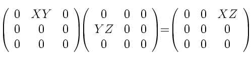
Thus multiplication is also preserved, and the symmetry transformation on the free density matrices induced by the bound state density matrix transformation does preserve multiplication among the free state density matrices as well as multiplication among the bound state density matrices.

.

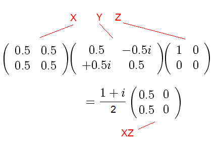
The Snuark Correction: In fact, the above product (XY) (YZ) is not equal to (XZ), but instead is a complex multiple of XZ. Part of the difference is that XY and YZ are not pure (non Hermitian) density matrices because they are not normalized; 2XY and 2YZ are correctly normalized. Even fixing this, however, there is a missing factor of sqrt(2) and a complex phase.

The detailed calculation can be computed by multiplying the 2×2 Pauli algebra spin projection matrices for spin in the X, Y, and Z directions. By associativity and idempotence we have XY YZ = X(YY)Z = XYZ, but instead of having XYZ = XZ, we need an extra factor of :

These sorts of calculations can be systemitized. They form the “snuark algebra” discussed in a previous post, The Sunark Algebra as a QFT in the context of the Koide mass formulas. Posts before and after that one give various calculational tricks that those who wish to master this sort of quantum calculations may find useful. Uh, the links to the preceding and following posts are up at the top of the post, between the banner and the date.

If we were using Schwinger’s normalization strategy, we would have that XY YZ = XZ and life would be easier, but we could not calculate geometric corrections to these sorts of products, and, for example, we would be missing the square root of 2 in the Koide mass formula.

We have shown how to embed the free states in the model of the bound states. We have shown that the exponential transformation by the bound states produces a symmetry operation on the combined bound and free states. And we’ve shown that this symmetry operation preserves the multiplication and addition on the free states.

Our embedding has created a new algebra, an algebra that combines the free and bound states. In moving from the free density matrix algebra to this combined density matrix algebra, we have altered the original, free density matrix algebra in the following ways: (a) we have added new quantum states, that is, the bound states, and (b) we have added new symmetry operations on this larger set of states.

It is possible that the process can continue. IF we can find bound states of our combined states (say, “n” of them) in the form of Feynman diagrams similar to the Feynman diagrams for the proton as a bound state of quarks, we can write these new “composite-composite” combined states as nxn matrices of the combined matrices discussed in this post. We can embed the combined states of this post in those matrices in the same manner we did in this post. And we can exponentiate the new composite-composite states to produce symmetry transformations on the combined matrices of this post.

The results of such a composite-composite theory will be a theory with yet more quantum states and yet more symmetries. Eventually the process will halt as we will run out of bound states that are suitable for modeling with qubits. At that time, if we have gone far enough, we may have an algebra of quantum states where ALL the symmetries of the quantum states are generated by the quantum states themselves.

E8 as the Limit of Bound State Density Matrices

E8 is most simply described as the simple Lie group that is a group of symmetries of its own Lie algebra. “Simple” means that there are no normal subgroups. A normal subgroup is a subgroup N that is preserved by the map for every g in the group. In the construction shown here, the most obvious possible normal subgroup is the free states. To see if this is a normal subgroup, we have to check to see if there is a symmetry that mixes free states with bound states. I suspect no such symmtry exists.

Even in the event that there is no such symmetry, and therefore the full algebra is not simple, all the various symmetries apply to the final bound states, that is, the most composite of the states, and I suspect that this is a simple subgroup, and therefore can be suspected to be E8.

I will probably write another post in this series showing how one can convert a known symmetry of a set of density matrices into a new “bound state”, that is, a matrix of the density matrices that is also a density matrix. But without a physical model, one cannot be certain that such a state would truly be bound.