Unitarity and the CKM Matrix

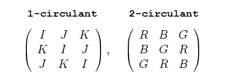
I’m busily working on writing the CKM matrix in Kea’s form, that is, as a unitary matrix that is the sum of 1-circulant and 2-circulant matrices. With the MNS matrix this was easier because I could begin with a unitary matrix, but the CKM matrix is usually given in absolute value form.

Looking through the literature, I’ve found a beautiful paper that digs to the core of the unitarity problem for the CKM matrix: A new type fit for the CKM matrix elements, Petre Dita, hep-ph/arXiv:0706.3588:

Abstract: The aim of the paper is to propose a new type of fits in terms of invariant quantities for finding the entries of the CKM matrix from the quark sector, by using the mathematical solution to the reconstruction problem of 3 x 3 unitary matrices from experimental data, recently found. The necessity of this type of fit comes from the compatibility conditions between the data and the theoretical model formalised by the CKM matrix, which imply many strong nonlinear conditions on moduli which all have to be satisfied in order to obtain a unitary matrix.

Dita’s CKM matrix estimate is:

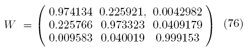
This needs a little explaining, probably.

Pop quiz! Spin Powers, and latest MNS news

I’ve been working on a derivation of the tribimaximal MNS matrix from first principles. It looks like it will require an assumption that the underlying particles follow a set of mutually unbiased bases (MUB). The calculation involves spin products. These are messy to compute unless you know some tricks I’ve discussed here previously.

So, did I waste my breath? Is teaching how to compute these things like shouting down a well? Let’s have a contest. First person to solve the following problem gets a $50 prize:

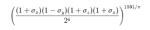
“Solve” means to write the above in reduced closed form in the comments section. The solution must be exact, for example, it must use rather than some numeric approximation such as 3.14159. Now I’ve chosen the values so that it will be easy to do with the techniques shown here, but will cause problems with mathematica or other automatic assistants. So go for the glory! Of course the winner can also ask that the prize be donated to a needy physicist such as Marni Sheppeard.

Meanwhile, I’ll share a few lines on what I’m doing with spin sums and the MNS matrix.

Book Review: My One Contribution to Chess, F. V. Morley

The Crossroads chess club provides me with the entertainment of watching chess games, along with the discussion that is natural to accompany such. Only rarely does my excessive kibbitzing force me to accept a challenge to play; though I have been practicing with such books as 1001 Brilliant Ways to Checkmate, my ability is somewhat lacking (too much mathematics, perhaps, which spoils one by allowing one to easily retract errors). My feeling is that chess is like football. It’s relaxing to watch a game but far too much effort to play. If I’m going to endure an hour of aggravation, memorize sequences of play and their likely chance of success, suffer nervous sweat until it drools down from my armpits to my belt, and run up my heart rate, I’d like to reach orgasm at the end of it. And with much better odds than the (under) 50% I achieve at the chess club.

Anyway, while observing a game, Nathan Jermasek (perhaps with the object of quieting my comments) handed me a slim book by F. V. Morley, “My One Contribution to Chess,” the subject of this book review. It should probably be noted that F. V. Morley and his book are supposed to be fictional creations of Stephen Potter in his famous 1952 book on gamesmanship, at least according to Wikipedia’s entry on fictional books:

You can’t buy My One Contribution on Amazon at the moment, but you may be able to find a used copy if you look around a bit. Perhaps eBay once caught a whiff of one.

Does the book exist or not? It’s hard to say, and certainly I’m not going to “correct” wikipedia on this. But the choice of the name F. V. Morley is interesting in that it leads to some mathematics which might vaguely have something to do with the physics we’re working on around here.

Electroweak unification, Quarks

To recap the previous post we began by combining the SU(2) spin-1/2 and U(1) operators into 2×2 matrices. We then showed that the leptons were solutions of the idempotency equation UU = U for 2×2 matrices subject to the additional requirement that the solutions be eigenstates of electric charge Q. For pure density matrix formalism, individual particle states are represented by primitive idempotents (with trace = 1), so we then converted these idempotents into primtive form by embedding them into 4×4 matrices. In doing this, we found that the idempotents given by the 2×2 matrices were composite, each being composed of two sub particles.

1-Circulant and 2-circulant matrices

In this post, we add the quarks to the picture. To do this, we need to use the 1-circulant and 2-circulant 3×3 matrices Kea talks about. We will write the general 1-circulant and 2-circulant matrices as follows:

Where I, J, K, R, G, and B are complex numbers. Note that there are only 6 complex degrees of freedom in the 1-circulant and 2-circulant matrices, one cannot create an arbitraray 3×3 matrix, with 9 complex degrees of freedom, from 1-circulant and 2-circulant matrices. In addition, setting R=G=B=1 gives a matrix of 1s, the same as setting I=J=K=1. Consequently, the 1-circulant and 2-circulant matrices together, have only 5 complex degrees of freedom, about half that of the 3×3 matrices in general. Writing a 3×3 matrix as a sum of a 1-circulant and a 2-circulant matrix is very restrictive; to write it as just a 1-circulant is even more so.

One obtains the basis for these matrices by setting one of the elements to 1 and the rest to zero. For example, putting I=1, J=0, K=0 gives the unit matrix. These 3×3 basis matrices correspond to permutations on three elements. We will think of the three elements being permuted as red, green, and blue, hence the labels R, G, and B for the 2-circulant matrices (i.e. R labels the permutation that leaves red unchanged and swaps green and blue, etc.). Similarly, “I” labels the permutation that leaves nothing changed, while J and K are the non trivial even permutations.

Electroweak Unification, Leptons

Quarks will require 1-circulant and 2-circulant matrices. Before adding that complication, let’s unify the lepton quantum numbers. Two quantum numbers (other than generation) distinguish quarks and leptons, weak hypercharge and weak isospin . Weak hypercharge is a U(1) quantum number; it has only one generator and therefore is commutative. Weak isospin arrives in two representations, singlets and doublets. The singlets have weak isospin quantum number of 0 and so we can represent them with any sort of 0. The doublets have spin-1/2, which we represent with the Pauli spin matrices:

There are three Pauli spin matrices, and they are linearly independent, so complex multilpes of them give 3 complex degrees of freedom. Since complex 2×2 matrices have 4 complex degrees of freedom, there is 1 complex degree of freedom left, the unit matrix:

The unit matrix is a natural basis for a U(1) symmetry, so we can combine weak hypercharge with weak isospin into 2×2 matrices. The number of degrees of freedom in the 2×2 matrices is just sufficient to support an SU(2) spin-1/2 and a U(1). Given a representation of an SU(2) operator, and a U(1) operator, the 2×2 matrix representation is simply the sum of the Pauli matrix representation of the SU(2) operator, and the U(1) value times the unit matrix. Similarly, given an arbitrary 2×2 matrix, we can split it into a U(1) portion and the SU(2) portions:

The above allows the weak hypercharge and weak isospin operators to share a 2×2 matrix representation. To unify the states, we have to pass to a density matrix representation.

Given a normalized quantum state vector (a,b), the density matrix representation of the state is a 2×2 matrix:

Similarly, given a U(1) state , we can convert it into a 2×2 matrix. For qubits, such a (pure) density matrix would be boring, it would only be the unit matrix. But for wave functions that depend on position, the density matrix is not trivial and contains the relative phase information of the quantum state (which is the only phase information that is physical). But for this post, simply note that 2×2 matrices are rich enough to contain both types of quantum numbers. A density matrix is partially characterized by the fact that it is idempotent, that is, . This characterization is not complete in that the equation has other solutions, in this case , and . These other solutions have trace 0 and 2, the usual pure density matrix has trace 1. It turns out we need these other solutions so their having the wrong trace is an issue. Further down we will show how to convert the traces to 1, but for now let us postpone the discussion.