Monthly Archives: December 2007

Mass Ends Year on High

WordPress’s management software reports that this blog has steadily increased its readership this year, with each month better than the previous:
Mass Blog hits, monthly chart, 2007

Happy New Year to the readers.

 My resolution is to be more professional about physics in 2008. And hopefully to retire.

5 Comments

Filed under Uncategorized

The Painleve Equations of Motion

In the general theory of relativity, the orbits are given by geodesics. A geodesic is a path that extremizes the path length. The path length is defined as the integral of ds over the path, where ds^2 is the metric. For the case of Painleve coordinates on the Schwarzschild metric, ds^2 is given by:
Painleve coordinates ds2
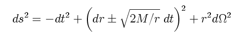
. Let’s let our path start at time t=0 and end at time t=1. For the path to be a geodesic, we must extremize the following integral (I’ll quickly sneak in a minus sign to make the path be timelike instead of spacelike):
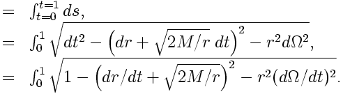
ds integral for Painleve coordinates
To make life easier for us, we will make the assumption that the orbital motion is in the \theta = \pi/2 plane so there’s no \theta dependence. That turns the angular part of the square root into r^2\;(d\phi/dt)^2 . Furthermore, since the simulation is going to use Cartesian, (x,y) coordinates, we might as well replace
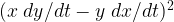
 r^2\;(d\phi/dt)^2 with (x\;dy/dt-y\;dx/dt)^2 , and dr/dt with x\;dx/dt + y\;dy/dt , their Cartesian equivalents. And put M=1, we can always fix it later by dimensional analysis.
Continue reading

5 Comments

Filed under gravity, physics

Painleve Coordinates

In the previous post, we took a tour through the literature and found that when general relativity is translated into the elegant mathematical language of the geometric algebra, the natural coordinates for a black hole turn out to be Painleve or Gullstrand-Painleve coordinates instead of the more common Schwarzschild coordinates. Our next post will derive the equations of motion for orbits in this coordinate system, but before we get into the difficult mathematics, we should take a quick look at the Painleve coordinates.

First of all, most of my readers will know that in general relativity, the choice of coordinates is quite arbitrary. Both Schwarzschild and Painleve coordinates describe the same object, the gravity field of a gravitating object which is spherically symmetric (and therefore non rotating), i.e. they are all descriptions of the black hole. In this sense they correspond to the same solution to Einstein’s field equations, which is sometimes called “Schwarzschild’s Solution”, or the “Schwarzschild Metric”. This is a little confusing, “Schwarzschild” was the person who found the Schwarzschild metric and he found it using the Schwarzschild coordinates, so his name is used twice here.

I guess I should put a pretty picture from the gravity simulation that resulted from all this here so it will show above the fold. This is a set of “knife edge” orbits, that is, orbits that quite nearly fall into the black hole but do not. Due to the time spent near the black hole, whose event horizon is marked in gray, the test masses get huge precession:
Knife Edge orbit example
We will be discussing the less pretty, but more mathematical subject of Painleve and Schwarzschild coordinates in this post.

Continue reading

1 Comment

Filed under gravity, physics

General Relativity, Painleve and QFT

The first problem in writing gravitation as a particle interaction is the fact that QFT works best on flat space, while general relativity is almost always written in arbitrary coordinates. One of the underlying principles of general relativity is that coordinates shouldn’t matter (background independence), so this problem appears to be a deep one. The point of view we will take here is that of the “new physics” .

That is, we will treat the equations of the old physics with more respect than we treat their theories. Consequently, instead of chasing after will-o-the-wisps like background independence, we will instead search for a method of writing general relativity using the mathematical tools of quantum field theory. Very fortunately for us, that method has already been found; it is the gauge theory of gravity discovered by the Cambridge Geometry Algebra Research Group. The purpose of this post is to introduce the theory to those who have not yet been exposed to it, and to note that this gravity theory (which is identical to GR so long as you restrict your attention to stuff that happens outside of the event horizons of black holes) picks out Painleve coordinates as a natural flat space (and therefore QFT compatible) coordinate system for a non rotating black hole.

Those with a graduate education in physics are already familiar with the Geometric Algebra (GA) in that it is equivalent to the Gamma matrices used throughout quantum field theory. So a gravitation theory that is equivalent to general relativity, but is written with gamma matrices, is a natural starting point for a search for a unified field theory.

The primary proponent for the use of GA in physics (outside of QFT) is David Hestenes, who applied it to classical and quantum mechanics. As the introduction to GA article at the Cambridge Geometry group’s website puts it:

We believe that there are two aspects of Hestenes’ work which physicists should take particularly seriously. The first is that the geometric algebra of spacetime is the best available mathematical tool for theoretical physics, classical or quantum. Related to this part of the programme is the claim that complex numbers arising in physical applications usually have a natural geometric interpretation that is hidden in conventional formulations. David’s second major idea is that the Dirac theory of the electron contains important geometric information, which is disguised in the conventional matrix based approaches.

Now that’s a pretty big claim: that geometric algebra is the best mathematical tool for all physics. I will spend the rest of this post exploring this claim in the case of general relativity, and then tracing the consequences for a unified field theory.
Continue reading

6 Comments

Filed under gravity, physics

Kepler’s Symmetries and Newton’s DE

This is the first of a series of posts about gravity, and the java applet I wrote that simulates Newtonian and relativistic orbits around a (non rotating) black hole. We begin by discussing the relationship between Kepler’s observations and Newton’s universal law of gravitation.

Usually when you write a scientific applet, most of the effort is in the java coding rather than in finding the equations. That is very much true about Newton’s equations of motion around a black hole, which are very easy. His Law of universal gravitation is:
Newton's universal law of gravitation F = G m M / r r
where F is the force, G is the universal constant, M is the mass of the black hole (or other spherically symmetric gravitating body), and m is the mass attracted. We will simplify this. We will use units with GM = 1, let m << M, rewrite Force as mass x acceleration, choose Cartesian coordinates (x,y,z) so that r^2 = x^2 + y^2 + z^2 
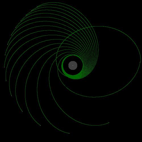
, only consider motion in 2 dimensions so z=0. The resulting simplified differential equation (DE) is:
Differential equation for Newton's gravity at black hole
Continue reading

2 Comments

Filed under gravity, physics

Regge Trajectories and Koide’s formula

As many of you know, I’m a proponent of the density operator formalism of quantum mechanics as opposed to the usual state vector / spinor formalism. The basic idea with density operator formalism is that quantum states should be represented by a density operator, or density matrix, rather than a state vector. This sort of idea is similar to the S-matrix theory that was part of the foundations of string theory, and I thought it would be worth exploring the similarities and differences.

The idea behind the state vector / spinor formalism is that quantum states are represented by state vectors or spinors. These sorts of objects are linear. In the state vector / spinor formalism, the spin state of an electron is typically represented by a Pauli spinor, a 2 element complex vector. Such a quantum state corresponds to spin-1/2 in some direction, \vec{v} = (v_x,v_y,v_z) . The operator for spin in this direction is typically written out as a 2×2 matrix using the Pauli spin matrices. One takes the dot product of the spin direction with the vector of Pauli spin matrices, giving:
Pauli spin operator in v direction

The spinor representing spin-1/2 in the v direction is a two element vector which is an eigenvector of the above matrix with eigenvalue +1. It is easy to see that for almost any 3 dimensional unit vector \vec{v} 
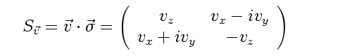
, such an eigenvector (in ket form) is given by:
Pauli spinor for spin 1/2 in direction v
The above formula gives a valid ket for any spin direction except (0,0,-1), but it isn’t normalized. To normalize it, divide by \sqrt{2+2v_z} . Higher spin states than spin-1/2, say spin-n/2, need spinors of size (n+1)x1 in size. So spin 3/2 will be 4×1 vectors, spin 2 will be 5×1, etc, but we won’t discuss these much.
Continue reading

13 Comments

Filed under physics

Mass and the New Physics

The previous few posts showed how a density matrix formalism gives a variety of quantum mechanics that naturally supports an interpretation of quantum states as symmetry operators on the quantum states. The method for doing this required ignoring the gauge bosons in bound states. For example, beginning with a complicated Feynman diagram for a bound state:
Feynman diagram for bound state of three particles
we simplified it by trimming off all the guage bosons and particle / anti-particle pairs created from gauge bosons. What’s left is just the valence fermions. We mark the points where these valence fermions change state with black dots and have:
Simplified bound state with just the valence quarks

This sort of thing will really annoy the old folks. It was the method we used to extend Koide’s charged lepton mass formula to the neutrinos. It may have something to do with the triality trick that Garrett Lisi used to fit the standard model particles to E8, and eventually we will return to the subject. But for now, I’d like to discuss the application of these trimmed diagrams as I was originally exposed to them; as a generic method of giving mass to massless particles. But first, a word about the philosophy behind the “new physics.”
Continue reading

4 Comments

Filed under Uncategorized