The Snuark Mass Interaction

In the standard model, the proton is made up of three quarks. The individual quarks are spin-1/2 particles. As elements of a QFT, the quarks are represented by propagators that satisfy the Dirac equation. What’s a bit odd is that the proton is also a spin-1/2 particle and is also represented by that same Dirac equation propagator.

Snuarks have a similar attribute. Three snuarks are (more or less) spin-1/2 particles and are represented by Dirac propagators. In the qubit representation, where we ignore spatial dependencies, their propagators are Pauli projection operators (i.e. density matrices). Somehow these three qubit objects combine to make a lepton or quark, which is also a qubit object whose (virtual) propagator is again a Pauli projection operator. In Feynman diagrams, what we are looking for is something like this:

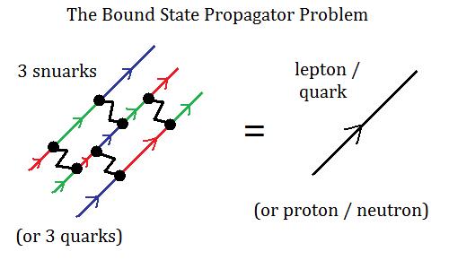
What we would like is a way of combining the propagators of the three snuarks into a single object that can fill the requirement of representing the propagator of the quark or lepton they combine into. This is the “bound state propagator problem” which we will return to more completely when we analyze the quarks. For the moment, let us consider the problem of how a bound state of three snuarks can model the lepton mass interaction that converts left handed leptons to right handed leptons and vice versa.

Mathematical Notes: Nonperturbative QFT

If the above talk of propagators as Pauli projection operators is unfamiliar, see equation (36) of the recent arXiv article: Quantum Electrodynamics of Qubits, or recent blog posts here.

As we’ve discussed before, qubit Feynman diagrams are finite to all orders in perturbation theory. This fact gives us a freedom unusual and unfamiliar in QFT: We don’t have to keep track of the orders of our Feynman diagrams. Everything’s finite.

In perturbation theory, it’s natural to write Feynman diagrams as polynomials in the coupling constant. As one desires a more accurate result, one includes higher terms in the polynomials. In qubit QFT theory, convergence is not an issue. Instead of organizing Feynman diagrams according to their order in the coupling constant, we will organize them according to how they modify the snuarks. Our solutions will be non perturbative. They will be nonlinear. And they will be exact.

Snuark Interactions

In the snuark interaction, a snuark absorbs (or emits) a “pregraviton” boson and changes color. There are 6 colors, three used by the left handed form, and three by the right handed form. For our example, we will orient the particle so that the left handed form uses +x, +y, and +z, and the right handed form uses -x, -y, and -z. In this text we will write these operators in their convenient and short algebraic form, i.e. (1+x)/2. If the reader prefers the traditional Pauli matrix notation, the six projection operators are as follows:

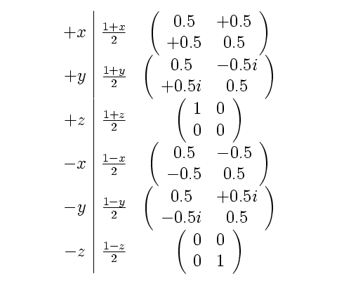
The right hand column is obtained from the middle column by substituting the Pauli spin matrices for x, y, or z.

A snuark interaction consists of an initial propagator, a final propagator, the interaction vertex, and the pregraviton boson propagator. For the moment, we will use an interaction vertex of “iq”. To include such a Feynman diagram in a calculation, we can replace the snuark propagators with the Pauli projection operator (from the table above), multiply by the interaction vertex, and add a boson propagator.

For the purposes of these calculations, we will not need to specify the boson propagator, but the reader is invited to imagine an appropriate spin-1 spinor, for example, where is the index for the spinor. Thus, as with the usual QED, the multiplication of the fermion propagators are handled in line in algebraic form (or in the traditional method with matrices), while the boson propagators connect together with indices.

Forbidden Transitions

Let’s suppose that the initial (left handed) snuark color is +x. There are three possible final (right handed) snuark colors, -x, -y, and -z. However, the propagators for +x and -x annihilate. That is, (1+x)/2 (1-x)/2 = (1-xx)/4 = (1-1)/4 = 0. Thus the +x to -x transition is forbidden, and similarly for +y to -y and +z to -z.

This leaves just six possible transitions for left to right snuark transitions instead of the nine otherwise possible. The Feynman diagrams and the associated algebraic values are:

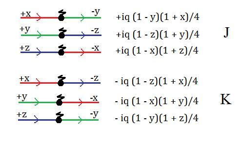
In the above, the initial and final propagators have not been multiplied out. For example, in the first line, the product of (1+x)/2 (1-y)/2 = (1+x-y-xy)/4. When calculating these sorts of things, remember that the letters are “matrices”. The squares of x, y, and z are 1, and different letters anticommute.

The Mass Interaction

The mass interaction is a point interaction, so we will assume that all three snuarks convert from left to right handed form at the same point, that is, all together. By the Pauli principle, no two snuarks can occupy the same state, so the final state, like the initial state, must include all three precolors.

This assumption implies that the snuark interactions can be grouped into two incompatible sets. These are labeled as “J” and “K” in the above. For example, if we took the +x to -y diagram from “J” and tried to combine it with the +y to -x diagram from “K”, we would find that we would need +z to become -z. This is a forbidden transition, hence snuark mass transitions come in only these two groups. If the +x snuark changes to -y, then the +z snuark must change to -z and the +z snuark must change to -x.

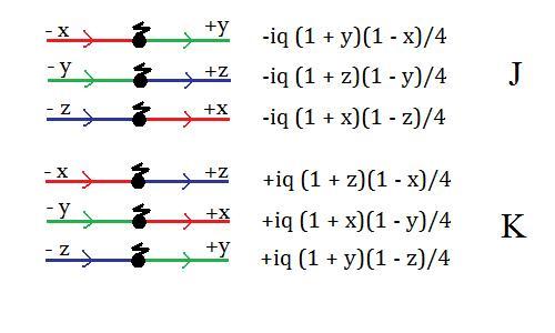
A similar set of snuark interactions take a right handed, -x, -y, -z, set of snuarks back to left handed +x, +y, +z form. We will label these according to how they permute the colors to match the left to right handed transitions:

The scalar parts of these snuark interactions, that is, the iq parts, can be factored out of a calculation. The Pauli algebra parts, the (1+x)/2(1-y)/2 parts, need to be connected up properly with other Pauli propagators. In the usual QFT calculation, we would specify real initial and final particle states with Pauli spinors, and these spinors would cap the ends of the Pauli matrices. For the case of three initial and three final Pauli spinors, the resulting calculation would give three chains of Pauli matrix multiplication. But we are not looking at a scattering calculation. Instead, we are looking for consistency relations for bound states and we will work entirely in the virtual particles (where the propagatos are density matrices, not spinors).

The Left to Right to Left Amplitudes

We have four interactions now. Two take a left handed set of snuarks and turn them into a right handed set. The other two do the reverse. The left and right handed states are independent. To get consistency equations it helps to eliminate either the left or right handed states. Arbitrarily, we will eliminate the right handed states: we will look at two consecutive mass interactions, the first from left to right handed, the second back to left handed. These are 6th order Feynman diagrams, but who’s counting, perturbation orders don’t matter to us.

For the left to right transition, there are two cases to consider “J” and “K” ; the same for the right to left transition. This means our left to left interactions will come in four types: “JJ” , “JK” , “KJ” and “KK” . For each of these interactions, there will be three chains of Pauli projection operators. There will be six factors of q. The imaginary unit i will appear six times, and there will be six factors of 1/4. But it’s natural to write these interactions with the factors attributed to the three matrix multiplications. The Feynman diagrams (with propagator arrows left off, they’re all to the right) and the corresponding algebraic amplitudes are:

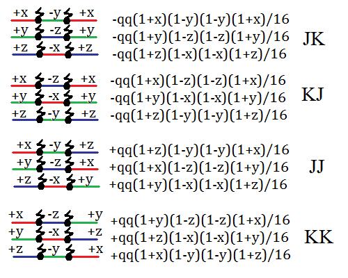
The 12 products of propagators in the above can be nicely reduced using the rules we’ve previously noted for the snuark algebra (or the reader can substitute Pauli matrices for x, y, and z). This can be written as nice pretty Feynman diagrams. Here’s the results of the calculations for the first product in the four JK, KJ, JJ, KK, cases:

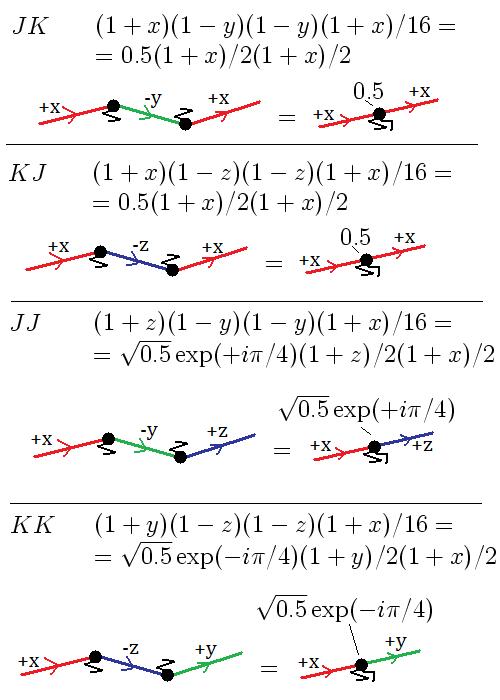
For example, in the JK calculation, the final result of (1+x)/2 is the propagator for a +x snuark, and so becomes the red propagator line in the Feynman diagram. The (1-y)/2 propagator, which gives the green propagator in the Feynman diagram, has been eliminated entirely in the reduced form. And there’s an overall scalar factor of 0.5 which we attribute to the “left to right to left” or “left to left” interaction vertex in the reduced Feynman diagram, which now has two pregraviton bosons coming from the vertex. (In the above, we have left off the “iq” vertex factors for clarity and cause we forgot them temporarily and don’t have the heart to redo the drawing.)

In each of the above four calculations, the left to right to left interactions have been converted into a left to left interaction with a modified vertex. When this is done, an extra scalar factor gets associated with the vertex. The scalar factor is 0.5 in the JK and KJ cases, and is 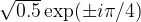in the JJ and KK cases. The reader can verify the vertex calculations by substituting in the Pauli matrices for x, y, and z, and the unit 2×2 matrix for “1”.

The upshot of all this is that we can convert our left to right and right to left interactions into more convenient left to left (or right to right) interactions if we change the iq factors associated with the vertices into (to account for the two iq s that we are pulling into one vertex), and include an extra complex amplitude (that corresponds to the phase picked up by the product of Pauli projection operators).

Since there are three Pauli projection operator multiplications for each of the JJ, JK, KJ, and KK cases, we’ve done 1/3 of the calculations we need. The others we can obtain by cyclically permuting {x,y,z}. This reduces the four left to right to left cases into four nice left to left amplitudes.

A Note to the Patient Reader

This is enough for one lesson / blog post. When I started writing this up, I thought that it would all fit in one post. And I guess it would if I wrote it at the usual high level where all the details are left for the reader to fill in. But filling in details is hard work and there is little motivation among my readers to work hard at understanding what a 50-year-old forklift driver is doing in elementary particles research.

So I’ve been trying to show the reader how to do the calculations at a detailed level. I want this series of blog posts to be a good introductory graduate level introduction to snuark QFT calculations because I think that the only way that physics can begin to use these ideas is if graduate students start using them. And the way to support that is to show detailed calculations, useful for understanding elemetary particles, that are as easily understood as standard QED theory. My goal is to make these calculations more clear, more understandable, than the calculations of any QFT textbook.