
Suppose we have an object X composed of three spin-1/2 fermions, R, G, and B. I should mention that “spin-1/2” means SU(2) here, in particular the usual 2-dimensional Pauli spin. The three fermions can each have spin +- 1/2, what spin states can object X have? This is a problem learned in undergraduate quantum mechanics; the answer is that 2x2x2 = 4+2+2, that is, one obtains a spin-3/2 quadruplet, and two spin-1/2 doublets. If that didn’t make any sense, then the wikipedia article on 2×2 = 3+1 spin might help, but this explanation is longer and better.
One easy way to derive the decomposition for n spin-1/2 particles uses Pascal’s triangle, and the fact that the simple representations of SU(2) have quantum numbers that run from -n/2 to +n/2, and have multiplicity 1 at each location. This fact is proved on Wikipedia in the usual method of the place (short and difficult to follow), but is probably well known to most of the readers. If we are to graph the quantum numbers of the various representations, we need one dimension, i.e. a number line, which we will draw horizontally. Then the various simple representations of SU(2) have quantum numbers as follows:
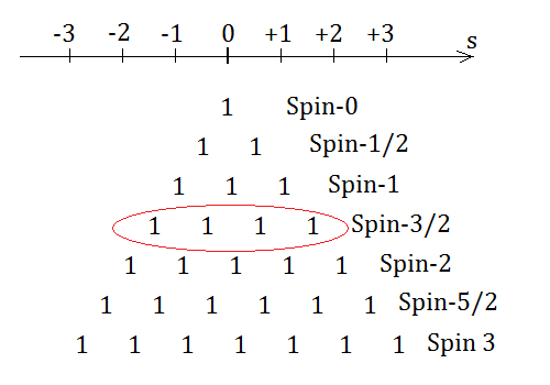
In the above, symbols “1” give the multiplicity of the eigenvalue. The spin-3/2 states, which are the “4” of 2x2x2 = 4+2+2, are circled in red. For the simple representations of SU(2) these are all the same so we could have used a dot, but farther down we’ll be dealing with higher multiplicities. Each representation is labeled by its highest spin state. The various representations have been assembled this way so that they are at least a little reminiscent of Pascal’s triangle.
Physically, when we combine N spin-1/2, SU(2) states, each of dimension 2, the result is a non simple representation of SU(2) of dimension 2^N. The undergraduate physics problem amounts to decomposing a product of representations into a sum of representations. If we didn’t care about the decomposition, or (as we will discuss later) this decomposition is inappropriate, we might instead decompose the product completely, into 2^N states, that is, forget about the SU(2) just think about the quantum states. The easiest way to do this (which is considerably easier than decomposing the product into the simple representations of SU(2)) is to use what are called the “basis states.”
The basis states are defined by simply taking the N contributing states, and choosing +1/2 or -1/2 for each. For three spin-1/2 states, the 8 basis states, and their spin eigenvalues, are as follows:
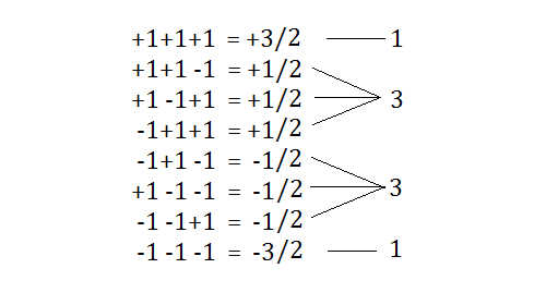
As you can see, the above mirrors the “3 choose n” row of Pascal’s triangle. And it should be easy to see that this is general, the multiplicity of the spin states for the product of N spin-1/2 systems will be given by the “N choose n” row.
So Pascal’s triangle gives an easy method of determining how N copies of spin-1/2 decomposes into simple representations of SU(2). For the case of N=3:
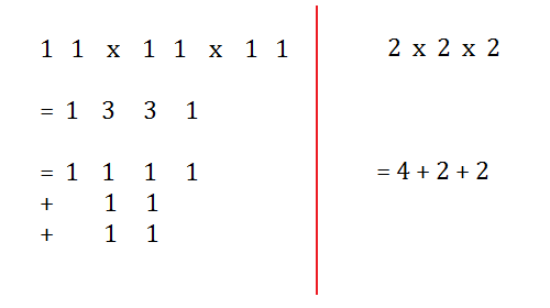
we find that 2x2x2 = 4+2+2, as mentioned above. Exercise for the reader: For N even, consider the product of N copies of spin-1/2. How many simple representations of SU(2) does this product decompose into?
Decomposing Symmetries
Elementary particle physicists work with symmetries of various accuracy. Some of the symmetries, such as spin (which is related to angular momentum and the fact that the equations of physics do not depend on orientation) are apparently perfect. There is very little experimental evidence against conservation of angular momentum and it is generally thought to be perfect.
When a symmetry is perfect, decomposing is completely supported and one does it automatically. For the 2x2x2 = 4+2+2 case, the four states in the “4” are closely related. Even though two of these states have spin +-3/2, while the other two have spin +-1/2, that is only a measurement of their spin in a particular direction (one usually assumes the z). The four states share the same total angular momentum and this distinguishes them from the two doublets.
An application of SU(2) where the symmetry is not perfect is “weak isospin.” Weak isospin breaks the elementary fermions into doublets and singlets. The right handed fermions are all singlets. SU(2) singlets have eigenvalue 0, so these right handed fermions all have weak isospin 0. The left handed fermions come in doublets. Following the conventions of SU(2), these states have weak isospin of +1/2 and -1/2.
Restricting ourselves to the first generation, there are two doublets. One is composed of the up and down quarks, the other is composed of the electron and neutrino. Surely the electron and neutrino are radically different particles and therefore weak isospin is a “broken symmetry” rather than a perfect SU(2) symmetry.
There is another way in which weak isospin is different from spin. With spin, one can arrange for particles that have spin oriented in any direction. In addition to electrons oriented as spin up or down, one also can find them, or arrange for them, to have spin north or spin west. In complete contrast, one cannot find a particle that is partly an electron and partly a neutrino. In theoretical elementary particle physics, this lack of intermediate states is called the result of a “superselection rule” 0710.1516, the particles separate into “superselection sectors” and there are no measurements or states that would correspond to the unobserved directions of weak isospin. Spin is an “external symmetry” of elementary particles while weak isospin is an “internal symmetry”.
So in the case of weak isospin, the utility of decomposition into simple representations is, only, well, weakly supported. Weak isospin is broken and is split by a superselection rule. In this circumstance, it makes sense, when dealing with preons that might contribute to the quantum numbers of the elementary fermions, to leave the decompositions at the level of Pascal’s triangle. This we will do, but first, let’s discuss weak isospin and weak hypercharge quantum numbers.
Weak Isospin and Weak Hypercharge
While weak isospin is an SU(2) symmetry, weak hypercharge is a U(1) symmetry. All the elementary particles, bosons and fermions, carry these quantum numbers and so they are expected to play an important part in any unification of the elementary particles. The elementary bosons correspond to transitions between certain pairs of elementary fermions and so their quantum numbers are defined by differences between pairs of elementary fermions.
For example, the W+ boson converts a left handed electron into a left handed neutrino so its quantum numbers are the difference between the quantum numbers of the other two. Another way of saying the same thing is that one can arrange (via suitable choice of antiparticle rather than particle) for the three pairs of quantum numbers to add to zero.
This fact, that the elementary particle interactions preserve quantum numbers and consequently when three particles interact one can arrange for a sum of three sets of quantum numbers to give zero is used in Garrett Lisi’s article “An Exceptionally Simple Theory of Everything, 0711.0770 which also discusses weak hypercharge and weak isospin at great length. In his paper, weak isospin is called 


For reference, a table of weak hypercharge and weak isospin quantum numbers for the elementary fermions:
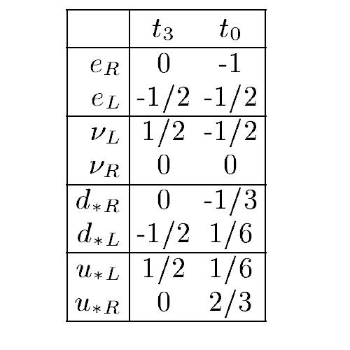
Note that the above give the quantum numbers of the particles. The antiparticles have quantum numbers that are the negatives of the above, with left traded for right; adding them to the list doubles the length to give 16 possibilities. In addition, the up and down quarks each come in 3 colors, which we will call red, green, and blue, and accounting for their multiplicity triples the 8 quarks giving 8×3+8 leptons = 32 elementary fermions. As an aside, note that these are for the first generation. The other two generations have the same quantum numbers but larger masses.
Let us examine the quantum numbers of the 8 elementary fermions which have weak isospin = 1/2. I will follow Lisi’s notation and use 
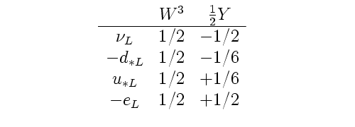
Given that the multiplicities of the quark states are triple, the above weak hypercharge quantum numbers are evenly spaced and suspiciously like a 1331 line of Pascal’s triangle. This naturally suggests that these 8 particles could be modeled as composites built from three subsidiary fermions (which, following tradition, we will call “preons” ) that come in a weak isospin doublet. Following the Pauli exclusion principle, the three preons have to be distinguished by a quantum number. The same problem, years ago, for the quarks, led to the postulate of color. Here it would be precolor.
Spin and Clifford Algebras
Since so much of elementary particle physics is built from the use of symmetries, it is only natural that spin is usually taught from the point of view of the symmetries of spacetime. It makes a good first step. However, if one’s objective is to continue Einstein’s search for physics in terms of geometry, it makes more sense to examine spin in terms of the Clifford algebra of the manifold of spacetime.
Spacetime has 3+1 dimensions, three spatial dimensions and one time dimension. We will use the +++- signature choice so in computing squares of vectors, the spatial dimensions will carry positive signature so 

In quantum measurements, noncommutativity arises from the fact that the order in which measurements are made matters. The simplest noncommutativity is anticommutativity, so we will assume that xy = -yx, xz = -zx, yz = -zy, xt = -tx, yt = -ty, zt = -tz.
The definitions we have made above, define a “presentation” of an algebra. That is, we define the “free algebra” over the symbols x, y, z, and t, subject to the rules 
Another geometric approach to the Dirac algebra is that of David Hestenes and his Geometric Algebra. In either case, spin arises directly from the geometry of spacetime. And the Dirac algebra is of dimension 4. Thus it contains two copies of spin-1/2 particles; this is how Dirac predicted the existence of the positron. He wrote the simplest equation (using the Dirac algebra) to model the electron and he ended up with two extra states that he concluded would be the same mass but opposite charge; the positrons.
And so it is a little attractive to try and derive the other quantum numbers from Clifford algebra states. To do this, requires that we understand what the quantum numbers of a Clifford algebra look like. To make what can be a somewhat long story short, one finds that the quantum numbers appear in hypercube form, that is, they are of the form (+1,+1,+1,…,+1) where any signs are possible and the number of dimensions is the dimensionality of the hypercube. As the number of basis vectors for the Clifford algebra increases, the number of dimensions to the hypercube also increases, but more slowly. This form of quantum number reminds one of the E8 quantum numbers used by Lisi; see table 8, page 17 of Lisi 0711.0770 where the 128 sized subset, “
N-Dimensional Pascal Triangle
For the case of the Dirac algebra, as implied above, the hypercube has dimensionality 2, and the quantum numbers of the Dirac algebra come in pairs. Thus the electron and positron, spin up and spin down, are modeled together. Since we have two dimensions, to compute the cross products of Dirac particles we need a two-dimensional Pascal triangle. To see how this works, let’s do a few calculations. Begin with the product of two Dirac particles:
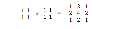
The calculation for three Diracs gives a pretty broad hint to the general solution:
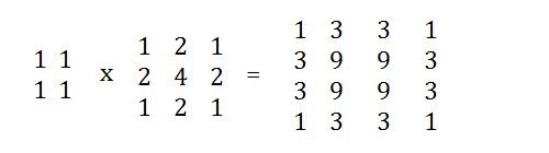
More generally, with N Dirac particles, the multiplicity for the state (n,m) will be the product of the corresponding Pascal triangle entries: (N choose n) x (N choose m) = (N!/(n!(N-n)!)) (N!/(m!(N-m)!)).
Weak Hypercharge and Isospin as Preons
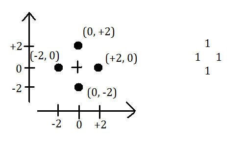
When one plots the weak hypercharge and weak isospin quantum numbers one finds that they show up as a square, but at a 45 degree angle to the axes:

From here there are several ways one can go on to try to fit the elementary particles. In the past, I’ve figured that the cube should define the axes for the natural quantum numbers. The basic ideas were explained in a paper I wrote up several years ago, The Geometry of Fermions (2004), but is better and more accurately described in later stuff that relies on density matrix theory implemented in Clifford algebra. However, in doing this I’ve not found a decent way of deriving mixing angles and all that.
Now I’m considering another model. In either case, the two basic problems are (a) there are too many states allowed by the Pascal’s triangle principle, and (b) the states are perfectly symmetric. Fortunately there is an obvious way to use break the symmetry, and reduce the states: While the quantum numbers of the Dirac algebra form a nice symmetric square, the interpretation of those quantum numbers is not at all symmetric. One of them gives the spin of the electron / positron. The other gives the charge. Similarly for more general Clifford algebras, so long as they are related to the spacetime manifold. Approximate symmetry and the breaking of that symmetry is natural in preons models like these.
New 12 preon / antipreon Model
Assume that there are 24 preons that can be grouped into 12 pairs of (preon,antipreon), only one of which can be put into any given elementary fermion which is made of a total of 12 of these preons/antipreons. A potential elementary fermion is defined by a choice of the preon/antipreon so there are 
In a sense, this amounts to summing over six copies of the Dirac algebra. Each of these copies has two preons and two antipreons with quantum numbers as follows:
A/B: (+1,+1) / (-1, -1);
C/D: (+1,-1) / (-1, +1);
For example, we can suppose that A and C are preons, while B and D are antipreons. Or B could be the preon and A the antipreon. Or whatever. It’s easy to compute the four possible quantum numbers from the above two pairs. We pick one from the A/B pair and one from the C/D pair and add quantum numbers together. There are four possible cases, and there quantum numbers are:
AC: (+2, 0);
AD: ( 0,+2);
BC: ( 0,-2);
BD: (-2, 0);
When we plot these, the usual square of Clifford algebra quantum numbers becomes rotated by 45 degrees, as desired:
What we’ve done above is transformed the four Dirac algebra states into four composite states that are rotated by 45 degrees from the original axes. We now can use the same techniques used above to compute the squared Pascal’s triangle. To cover the 32 cases used by the standard model fermions, we need six of these squares. This implies that the elementary fermions are built from 6×2 = 12 subpreons, chosen from preon / antipreon pairs. Taking the 6th power of the above, one obtains the square of the 6th row of Pascal’s triangle, tilted 45 degrees. In the drawing, the states that are left after symmetry breaking are shown in red:
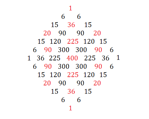
If the above were drawn without the preon / antipreon restriction, it would have the usual square form but with many times as many states shown. A new forbidden state would appear in the center of each diamond, and these would extend out to fill the overall diamond shape out to be a square again. In this way the reader can see that even a very simple symmetry breaking mechanism can drastically reduce the number of states available and the shape of those states. In the above, the scope of the states have been reduced, and their multiplicity has been vastly reduced. In addition, only the “even parity” states remain. The odd parity states are the centers of the diamonds.
While the Dirac algebra needs two quantum numbers to define its states, the actual quantum numbers are somewhat arbitrary with three choices. The quantum numbers are all +-1s and their operators commute, so these are multiplicative quantum numbers. Instead of spin S and charge C, one could instead use spin S and “spin X charge” SC. Or C and SC. For larger Clifford algebras the number of choices increases quickly. For the Dirac algebra, this amounts to the assumption that one take a particle from preon / antipreon pairs, but it is conceivable that a generalization to the next larger Clifford algebra will give nontrivial results.
The next step in the symmetry breaking will be to eliminate 2 of every 3 columns. Of course the model I’m working on involves “snuarks” which are Mutually Unbiased Bases (MUBs) taken from the Pauli algebra. The basic idea of a MUB is that the elements of one MUB and another have transition probabilities that are all equal. This seems to require that the 3 MUBs have identical composition as otherwise they would be unbalanced.
Generations and Bosons
There are two other parts to the puzzle, the generation structure and the bosons. In this preon model, these two problems are handled together. As noted in my many previous blog posts, the Koide mass formulas can be derived in density operator form. The “valence” preons do not depend on generation and are modeled as the usual Hermitian pure density matrices. The boson that modifies a preon represented by a density matrix V into a preon represented by a density matrix W is represented by the non Hermitian pure density matrix 2VW (which formula works only if V and W are taken from two different MUBs, the “2” comes from the transition probabilities of the Pauli MUBs, which are 1/2).
These boson states represent the changes to the valence preons. The bound state is represented as a matrix of density matrices and one solves the primitive idempotency equations to find the possible bound states. For a given set of valence preons, one finds that there are three solutions, these correspond to the three generations.
In this model, one has interactions as two fermions and one boson. Do the quantum numbers sum to zero as used in Lisi’s model? Yes, they do, as can be seen by looking at a simple example taken from the Pauli MUBs. Let X = (1+x)/2, Y = (1+y)/2 be the density matrix operators for spin in the +x and +y directions. Their quantum numbers with respect to x and y are +1 and +1, respectively. The representation of the boson that converts one to the other is 2XY = (1+x)(1+y)/2 = (1+x+y+xy)/2. Thus the (x,y) quantum numbers are as follows:
X: (1, 0),
Y: (0, 1),
XY: (1, 1),
and the quantum numbers add, as required.
Some of my readers might have noted that this post is a lot easier to understand than my usual. The first draft started out from the Cliford algebra point of view, but before I finished it, I got to talking with one of my buddies, Forrest LeDuc, over at the Overlake Chess Club about the theory. For his level of mathematics, the squared Pascal’s triangle was the right way to explain it, so I wrote it out with a pen on the Seattle Post-Intelligencer I customarily read while watching chess games there. And then I realized that that’s the way the blog post should be organized. I’ll add the Clifford algebraic details in another post, later.

Pingback: Chess Board » Pascal’s Triangle and Lisi’s E8 Quantum Numbers
Thanks for this very interesting post, Carl. This gives me a lot of clear, vital facts, although quite a lot of it is far too mathematically abstract and physically abstruse for me. Firstly, isospin is very abstract. What physically is the isospin charge?
I know historically Heisenberg is supposed to have suggested isospin symmetry in 1932 when the neutron was discovered, because neutrons and protons (nucleons) had apparently identical nuclear properties and very similar masses, despite having grossly different net electric charge.
So isospin charge was at first supposed to be the strong nuclear charge that binds nucleons together in nuclei. Then after the Yang-Mills theory was invented and used to improve Fermi’s theory of beta decay, isospin was the name for the weak interaction charge.
But what about weak hypercharge, which is so closely related to the electric charge in the Standard Model?
Wiki page you link to, http://en.wikipedia.org/wiki/Weak_isospin makes a very interesting claim:
“W^0 boson (T_3 = 0) would be emitted in reactions where T_3 does not change. However, under electroweak unification, the W^0 boson mixes with the weak hypercharge gauge boson B, resulting in the observed Z^0 boson and the photon of Quantum Electrodynamics.”
The key thing here is the mention of the “weak hypercharge gauge boson B”.
So the electroweak theory U(1) x SU(2) doesn’t just have 1 + 3 gauge bosons (photon, W^+, W^-, Z^0), it has also a B hypercharge gauge boson!
But isn’t that identical to the photon? How is the B hypercharge gauge boson supposed to differ from the photon? If it doesn’t differ from the photon, then surely it is the photon, and in that case electric charge (mediated by B bosons) would be indistinguishable from weak hypercharge.
I don’t see physically how U(1) is supposed to represent two things, electric charge and hypercharge, without having a separate gauge boson. If it has a separate gauge boson, then shouldn’t the standard model be written as U(1) x U(1) x SU(2) x SU(3), instead of U(1) x SU(2) x SU(3)?
The standard discussions in textbooks (I think it is in Weinberg, Zee and Ryder) say that hypercharge is fundamental and electric charge is just an aspect of that. However, they don’t provide any physical evidence for that view so it’s just a belief. The Standard Model has been formed as a combination of U(1) electromagnetic, SU(2) weak isospin, and SU(3) colour charge gauge interactions, plus some form of Higgs field to provide mass and electroweak symmetry breaking.
I don’t see how (as Wikipedia claims): “W^0 boson mixes with the weak hypercharge gauge boson B, resulting in the observed Z^0 boson and the photon of Quantum Electrodynamics.”
This sounds very vague and speculative to me. Is there any physical evidence for it? Surely the W^0 is just a label for Z^0? I know that evidence for the Z^0 (neutral currents, involving exchanges of Z^0 gauge bosons between charges) was discovered experimentally in the 1970s, and that in 1983 CERN discovered concrete evidence for the Z^0, W^+ and W^- weak gauge bosons, but what about the alleged weak hypercharge gauge boson, B? Is there any direct evidence for B?
It’s pretty sad that it’s hard to distinguish the fact based physics from the speculation in the Standard Model. It’s all treated alike in textbooks.
I can grasp how SU(N) gives rise to a matrix of N x N gauge bosons, e.g. red, blue, green for N = 3 gives the following 3 x 3 matrix for SU(3):
{red-antired, red-antigreen, red-antiblue}
{green-antired, green-antigreen, green-antiblue}
{blue-antired, blue-antigreen, blue-antiblue}
or
{r-ar, r-ag, r-ab}
{g-ar, g-ag, g-ab}
{b-ar, b-ag, b-ab}
I can even grasp physically why these 9 gauge bosons are too many for any real interaction between two charges (one of the gauge bosons can’t have the right colour combination to contribute in any given interaction, so it appears colourless and only 8 can effectively contribute, http://math.ucr.edu/home/baez/physics/ParticleAndNuclear/gluons.html ).
Applying this to SU(2) gives the following. Weak isospin charge has values of +1/2 and -1/2. Therefore the 2 x 2 matrix of gauge bosons for SU(2) should be:
{+1/2 – 1/2, +1/2 + 1/2}
{-1/2 -1/2, -1/2 + 1/2}
=
{0, +1}
{-1, 0}
So two of these are zero-isospin gauge bosons, which are clearly the same thing, so the 4 components of this matrix only give 3 distinct elements: 0, +1, and -1 isospins.
Then the W^0 or Z^0 gauge boson is that with 0 isospin, the W^+ gauge bosons have +1 isospin, and the W^-1 gauge bosons have -1 isospin.
There is absolutely no problem with this, which is experimentally confirmed. I just wonder whether weak hypercharge is real, or is just a mathematical transmogrification of the values of weak isospin and electric charge?
I don’t believe in U(1) x SU(2) as being an electroweak unification. If nature is simple, instead of having a 4-polarization photon as gauge boson for one kind of electric charge in U(1) as occurs in the Standard Model, you would need a theory like SU(2) which has two kinds of electric charge (positive and negative), with force fields mediated by charged gauge bosons. This will produce repulsion of unlike charges because the directly exchanged gauge bosons will make similar nearby charges recoil apart. Attraction of unlike charges then arises because of the unlike charges shielding and shadowing one another from charged exchange radiation from the rest of the universe. It can easily be proved from the vector sum that the force of attraction between unit unlike charges is equal magnitude but opposite in sign to that between unit like charges.
So it’s tempting to suggest that SU(2) with massless charged gauge bosons is actually electromagnetism. This merely requires the removal of U(1) electromagnetism from the Standard Model, plus a change in the Higgs field so that it doesn’t give mass to all charged SU(2) gauge bosons at low energy, only to a certain number of them at high energy so that weak interactions occur between particles with left-handed spin.
It’s interesting that charged massless gauge bosons can actually propagate in the vacuum as exchange radiation (because the magnetic field self-inductance gets cancelled out if such bosons are streaming in two opposite directions in the vacuum between charges), even though they can’t propagate along a one-way route in the vacuum due to infinite self-inductance.
Now, if we consider this carefully, for the massless gauge boson SU(2) you get electromagnetism from two charged gauge bosons, and the neutral, massless gauge boson of SU(2) can either play the role of weak hypercharge or of something else like gravity.
Initially I thought that it was the graviton, but now I’m wondering if it’s the weak hypercharge boson, B, if that is a physically real concept, and if the details work out; e.g. the mechanism I suggest for electromagnetism requires two charged gauge bosons, so the neutral massless gauge boson might well not have the right properties to give the physically known facts about weak hypercharge, although I’ve having difficulty finding any direct physical evidence of weak hypercharge.
Is there any evidence of weak hypercharge from Fermi’s theory of beta decay? The basic idea as summarised at places like http://hyperphysics.phy-astr.gsu.edu/hbase/quantum/fermi2.html doesn’t seem to physically invoke weak hypercharge.
If weak hypercharge isn’t a physical necessity from experimental evidence, knowing that would clear up my confusion and suggest to me that SU(2) with massless gauge bosons is the correct symmetry group for quantum gravity and electromagnetism, and allow concentration on a detailed predictive mechanism (to replace the Higgs theory) by which mass is given to such bosons to give rise to the left-handed weak force.
Great information on your site. I often link to your site when doing various Google searches and always appreciate your insight. There appears to be a lot of connections in the basic geometry of fermions and the geometry of logic (e.g. symmetry, rotation, reflection). I’m writing an encyclopedia article on Dr. Shea Zellweger’s work and his symmetry based X-Stem Logic Alphabet (XLA). His logic notation system allows you to manipulate whole truth tables easily and intuitively with simple flips and rotations. Additionally, he demonstrates the power of viewing the 16 connectives in four progressive spatial dimensions. The connections between the math, symmetry, rotations and reflections of two valued logic and the fundamental underlying structure of matter seem quite similar in many ways.
William,
Thanks for the comment. I’ll look up Shea Zellweger as soon as I get some time. I’ve saved the google search on my “favorites” so I don’t forget.
I made a living for a decade or two designing digital logic and the analogies to Karnaugh maps and truth tables was obvious to me while writing “The Geometry of Fermions”. And of course that was the reason for calling the preons “binons”, they follow rules of binary logic.
Carl, hope you don’t mind me throwing this in. I have developed a preon theory that starts from some basic assumptions and develops a preon-based bound state particle hierarchy from which I develop a formula for calculating mass. A number of fundamental features evolve from this. It may be total nonsense, or there may be something in it, be interested in some feedback. Can be downloaded as small PDF off my website at http://rupertgerritsen.tripod.com/pdf/published/A_Conjectural_Preon_Theory_and_its_Implications.pdf (also on Kindle)
Kind regards
Rupert