David Hestenes’ electron model

John R Ramsden, as a comment on Motl’s blog, points us to an article by David Hestenes, Reading the Electron Clock, 0802.3227. There are two good reasons for looking at this paper, and the experiment that inspired it. First, we can use it as an excuse to discuss Hestenes’ electron theory, and what it looks like in the density operator language. Second, in a later post, we can discuss de Broglie’s matter waves.

Zitterbewegung

As the Wikipedia Zitterbewegung article states, Zitterbewegung [German for trembling motion] is an “interference between positive and negative energy states produces what appears to be a fluctuation (at the speed of light) of the position of an electron around the median, with a circular frequency of , or approximately .” It was first noticed by Schoedinger, I think. It comes about when you compute the position operator, as a function of time, for an electron with momentum. The electron’s momentum p and mass m define a velocity v = p/m, and the position operator x ends up being given partly by vt = pt/m, but there is another term, an oscillatory term. [In quantum mechanics, the Hamiltonian H gives the energy, and setting H = mc^2, so the equation in the Wikipedia article looks like . Also, I’m mixing metaphors a bit between relativistic and non relativistic definitions of mass. Read the original articles for the correct derivation.] So long as you restrict to solutions of the Dirac equation which have only positive or negative energy, there is no Zitterbewegung, and this is how the frequency is usually ignored.

Hestenes is a long time advocate of The Zitterbewegung Interpretation of Quantum Mechanics. In his interpretation, Zitterbewegung (sometimes called zbw or zitter) is not due to interference between positive and negative frequencies but instead arises from the complex phase factor present in all quantum mechanics. Hestenes looks at the zbw as being associated with spin. The consequences are wide. He writes:

The essential feature of the zbw idea is the association of the spin with a local circulatory motion characterized by the phase factor. Since the complex phase factor is the main feature which the Dirac wave function shares with its nonrelativistic limit, it follows that the Schroedinger equation for an electron inherits a zbw interpretation from the Dirac theory. It follows that such familiar consequences of the Schroedinger theory as barrier penetration can be interpreted as manifestations of the zbw.

From my point of view, zitterbewegung corresponds to the frequency with which the electron switches back and forth from its left handed to right hand form. At its deepest level, it arises from the Feynman checkerboard model previously discussed and the requirement that the left and right handed fields are massless and travel at speed c. (So the electron must oscillate back and forth in order to be stationary.) Hestenes also sees zitterbewegung as arising from spin, but in a manner that is a little different from mine. And he also begins with geometric (Clifford) algebra so our models have deep similarities. To see where the differences come about, it’s useful to analyze Hestenes’ mathematics from my (density matrix) point of view.

Hestenes’ model in Density Matrix form

Where Hestenes and I differ is in that while he uses the state vector formalism, for which the geometrization is kind of complicated and a little arbitrary, I use the pure density matrix formalism, which has only one unique and very simple geometrization. For example, in spin-1/2 qubits, the natural density matrix (operator) form for a spin up quantum state is (1+z)/2 where {x,y,z} are the Pauli spin matrices. The quantum state for spin in the -x direction is (1-x)/2, etc.

To review the traditional relationship between pure density operators and state vectors [i.e. where the density operator is defined from the state vector rather than vice versa], let’s discuss the quantum state for spin up. We can write a state vector representation as |a), where the curved bracket is used to prevent WordPress from misinterpreting. This state vector is not unique, but may be multiplied by any complex phase to obtain an equivalent representative, as in exp(+ik) |+z). This is the “ket.” For each such there is also a “bra” which takes the negative phase: exp(-ik) (+z|. The density matrix form is given by the product:
(1+z)/2 = exp(+ik) |+z) exp(-ik) (+z| = |+z)(+z|.

Now the density matrix was very naturally geometrized (written in Clifford algebra with geometric interpretation) as (1+z)/2, but this does not define a unique state vector form. And so, of course, Hestenes’ geometrization of the state vector is also not unique. He must provide information that corresponds to that arbitrary phase. Since he is building a geometric theory, he must provide that information in geometric form.

I’ve been discussing this with the Pauli algebra (or the “Pauli Spin Matrices” if you absolutely have to perform the ugly and unnecessary act of choosing an arbitrary representation for the Pauli algebra), but the differences are general to all Clifford algebras and also apply to the Dirac algebra (i.e. Dirac’s gamma matrices), and I will switch back and forth between the algebras.

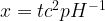
In Hestenes’ paper, the arbitrary complex phase is given by equation (34), . The origin of this arbitrary phase is better described in an earlier Hestenes paper, The Kinematic Origin of Complex Wave Functions, where it is defined on page 3 as follows:

The next step in explicating the geometric structure of the Dirac theory is to reformulate
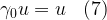
it in terms of the spacetime algebra. One easy way to do that is to choose a fixed unit
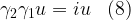
spinor u satisfying the eigenvalue equations


where i is the usual unit imaginary of the complex field. Equation ( 8 ) is especially signiciant because it relates i to the bivector , and thus reveals that i has an implicit geometric meaning in the Dirac theory. This meaning can be made explicit by eliminating i from the theory in favor of the geometric quantity . It is easy to prove that each Dirac spinor can be written in the form

where is a unique even element of the real Dirac algebra.

The real Dirac algebra is just the real Clifford algebra on x, y, z, and t. The even elements are the elements of the even subalgebra, that is, the subalgebra whose basis is {1, xy, xz, xt, yz, yt, zt, xyzt}.

Density matrices and the even subalgebra

Why is he talking about the “even subalgebra here?” It seems very arbitrary until you understand how the density operator language treats quantum states. A quantum state is given by a primitive idempotent of the Dirac algebra (which is a Clifford algebra). A complete set of basis elements means four quantum states that form a basis for any quantum state (just as two quantum states, spin up and spin down, form a complete basis set for a Pauli spin-1/2 state). In the density matrix language, these four states could be Q, R, S, and T which are 4×4 matrices that annihilate each other and sum to 1.

One finds complete basis sets for a Clifford algebra by first defining a “complete set of commuting roots of unity.” This means as large a set of operators (that square to 1) that we can put together, provided that they all commute and we don’t include trivial products. For the Dirac algebra, a complete set of commuting roots of unity is {ixy, ixyzt}. In fact, these are the usual set chosen for the usual spinors used in the Dirac equation. Note that they are both elements of the even Dirac algebra.

With this choice of the commuting roots of unity, the four states making up a complete basis set (electron, positron, spin up and spin down) is:
Q = (1+ixy)(1+ixyzt)/4,
R = (1+ixy)(1-ixyzt)/4,
S = (1-ixy)(1+ixyzt)/4,
T = (1-ixy)(1-ixyzt)/4.

More generally, we might want to look at spin in some other direction say w = ax+by+cz where . So “w” is another element of the Dirac algebra, a spatial vector. To get the basis set oriented in that direction, we need to replace the “xy” with something that has to do with u. Working in the +++- signature so that zz = +1, we can write xy = (xyz)(z). Thus for a general direction u, the complete basis set is:
Q = (1+ixyz w)(1+ixyzt)/4,
R = (1+ixyz w)(1-ixyzt)/4,
S = (1-ixyz w)(1+ixyzt)/4,
T = (1-ixyz w)(1-ixyzt)/4.
Note that the above is in the even subalgebra, the same place which Hestenes seems to arbitrarily pick out for . And it should be clear that considering all the possible directions, the above sorts of things cover the even subalgebra. For example, we can write 1=Q+R+S+T, and ixyzt = Q-R+S-T, and ixyzu = Q+R-S-T, and more difficultly, ut = Q-R-S+T. Thus we get the scalar 1, the pseudoscalar ixyzt, an arbitrary spatial bivector ixyzu, and an arbitrary space-time bivector ut is covered by the basis set. This exhausts the even subalgebra’s basis set, {{1}, {ixyzt}, {ixy, iyz, izx}, {xt, yt, zt}} so any even element of the subalgebra can be written as a sum over multiples of the pure density operators given above (which do not mix particle with antiparticle).

The arbitrary spinor u as “fictitious vacuum”

The other part of Hestenes’ Dirac wave function prescription is the fixed spinor u. It’s quite complicated, and the confusion associated with this has generated some interesting literature, see the excellent paper by Baylis, quant-ph/0202060. Hestenes goes through a lot of gymnastics to explain this arbitrary item, but in the context of density matrix formalism and Julian Schwinger’s measurement algebra, its meaning is quite clear. It is a choice of vacuum.

There are two Schwinger papers that define the fictitious vacuum. The first is The Algebra of Microscopic Measurements which is quite short and easy to understand. The vacuum is defined on the second page of the second article, The Geometry of Quantum States. The reader who finds the following discussion impossible to fathom might read Schwinger’s version. The difference is that his is written in a field theory language while I’m writing here in a wave function vernacular.

Spinors Defined using Ficitious Vacuum

Let’s work entirely in the density matrix formalism. We choose a (more or less) arbitrary pure state “V” and call it the quantum vacuum. Given a (pure) density matrix state Q, we define corresponding bras and kets as follows:
|q) = Q V,
(q| = V Q,
providing QV and VQ are nonzero. (If they are zero, then we go back and choose another vacuum. Schwinger covers this case more elegantly, by defining a new state outside of the universe of states, that does not annihilate anything.) Since Q and V are pure density matrices, they satisfy QQ = Q, VV = V, and tr(Q) = tr(V) = 1. We now show that |q) and (q| act just like kets and bras.

As a first step, let’s compute (q|q):
(q|q) =(V Q) (Q V) = VQV.
Now the state V is fully defined by the fact that it has some set of quantum numbers defined by a complete set of operators. As a pure density matrix, it has these quantum numbers double sided, that is, they apply to either side. But the operator VQV has V on both sides and so it will also be an eigenstate for these operators and it will have the same eigenvalues. Therefore, it is a multiple of the eigenstate V. To figure out the multiple, write v = tr(VQV). Then VQV = vV. The reader can see that v must be real because this is just the transition probability between the states V and Q, that is, tr (VQV) = (q|v) (v|q). This tells us how to scale our spinor definition. And it also tells us that in computing scalar products, our answers will be in multiples of the vacuum V.

Now, let M be an arbitrary quantum operator. We wish to compute its expectation value for the state Q. In the density matrix language, this is given by:
m = (M) = tr( Q M ) = tr (Q Q M ) = tr (Q M Q) which must be equal to our (q| M |q) so tr (QMQ) = m, and as before, QMQ = mQ. Using this fact:
(q| M |q) = (VQ) M (QV) = (V Q M Q V)
= (V (QMQ) V) = (V mQ V) = m (VQV) = mv V.
The “v” is just the normalization for our choice of vacuum. That is, (q|q) = v V so we need to divide by v. The result is that (q| M |q) = m, and our definitions of (q| and |q) give the same expectation values as usual.

So the arbitrary “u” that Hestenes’ model of the electron uses corresponds to the arbitrary vacuum choice that Schwinger introduces when he converts his measurement algebra into state vector form. It corresponds to a way of picking an arbitrary geometric phase when converting from density matrix form to a spinor form.