Berry ( or Pancharatnam-Berry or quantum ) phase.

Classically, if a vector is parallel transported around a closed circuit on a curved space, it returns with its orientation altered. A drawing modified from the one at the a review of Berry’s Geometric Phase on the web page of Nicola Manini (assistant professor at Milan University) shows the classical effect:

In the drawing above, when the red vector is parallel transported through the 13 marked points around the sphere (all on a spherical triangle), the vector returns rotated.

If the vector is considered as a 2-d object in the tangent space of the surface of the sphere, the rotation of the vector can be given by an angle. The angle that the vector is rotated by is proportional to the surface area of the spherical triangle. If the spherical triangle is built from three 90 degree angles, it is clear that the vector is rotated by 90 degrees, and, under the (correct) assumption that the rotation angle is proportional to the area of the spherical triangle, this tells us that the ratio of spherical triangle area to rotation angle is given by 1. That is, if the spherical triangle has surface area A, the vector will be rotated by the angle A. A similar effect occurs in quantum mechanics when a spin state is sent through a sequence of orientations. This is kind of interesting in that we are turning a measure of spherical area into an angle.

In the usual spinor representation of quantum mechanics, the phase of a quantum state is arbitrary; one can always multiply a spinor by a complex phase and the new spinor represents the same state.

Density matrices are simpler in that they do not carry arbitrary phase information and consequently we can discuss Berry phase very elegantly and easily in density matrix formalism, which is the subject of this post.

Phase in Quantum Mechanics

In quantum mechanics, phase appears in three ways, (1) the arbitrary phase which corresponds to the multiplication of a spinor by a complex phase , (2) the phase that a wave picks up when we consider it changing with position and time which we can write , and (3) geometric or Berry phase.

The arbitrary phase of spinors does not appear in a density matrix theory because it is cancelled out when one converts a spinor into a density matrix. Since density matrix theory and spinor theory give equivalent descriptions of quantum mechanics, it should be clear that the arbitrary quantum phase of spinors cannot be detected by experiment. So in working in the density matrix formalism we can avoid this source of phase completely. And if we consider a quantum wave value at only a single point in space and time we can avoid the second source of phase differences. So the natural formalism to discuss geometric phase is density matrices for qubits (or qutrits or whatever) considered at a single point in space and time. And this is what we will do, we will use the pure density matrices for spin-1/2, qubits.

As is usual on this blog, for the Pauli algebra, we will use x, y, and z for the three Pauli spin matrices. By keeping our notation algebraic, we will avoid the necessity of choosing a set of matrices to represent the algebra. This also means that our efforts will also apply to more arbitrary Clifford algebras.

.

Generalization to higher Clifford algebras
While we will be using the Pauli algebra, our results are quite general and apply to any Clifford algebra. Here we give instructions for applying these results more generally.

In a Clifford algebra, any two canonical basis elements (sometimes called “bilinears” as in Dirac bilinears) either commute or anticommute. Two operators that commute correspond to operators that can be simultaneously diagonalized and consequently are part of a complete description of a quantum state. In the Dirac algebra, an example of two commuting canonical basis elements would be and .

The structure of the commuting operators is interesting in that it defines the structure of the natural quantum numbers of the Clifford algebra. These are a hypercube as is discussed at more length in my 2004 paper The Geometry of Fermions.

For the purpose of this post, the more interesting case is when the two canonical basis elements do not commute (and therefore anticommute). From the example of the Dirac algebra, two canonical basis elements that anticommute is and . To make these equivalent to the Pauli algebra we need for them to square to unity. So if we’re dealing with a signature that leaves either of them negative, multiply them by i (which is why we are in a complex Clifford algebra).

Two such elements multiply to produce a third canonical basis element. These three canonical basis elements all anticommute with each other and they square to +1, +1, and -1. To make them a representation of the Pauli algebra, multiply the product by i. For the above example of the Dirac algebra, the resulting equivalence to the Pauli algebra (in the -+++ signature) would be .

More generally, any two anticommuting elements of a Clifford algebra generate a representation of the Pauli algebra. In such a representation, Berry phase can be calculated using the techniques discussed in this post for the Pauli algebra.

.

So let’s make the calculation. Let u, v, and w be three unit vectors. We will interpret them as matrices through taking the dot product with the Pauli spin matrices. So if u = (0.6, 0.8, 0), then the related algebra (or matrix) object will be 0.6x + 0.8y. This is the operator for spin in the u direction. And U = (1+u)/2, V = (1+v)/2, and W = (1+w)/2 are the three quantum states with spin in the u, v, and w directions. So we will slightly abuse our notation and let u stand for both a direction in 3-space and an element of the Pauli algebra, the operator for spin in the u direction.

Thinking of the state U in terms of the bra and ket language of spinors, we have , and . Therefore we have that U is a double-sided eigenstate of u: uU = Uu = U. We wish to consider the phase result from sending the quantum state through the directions u, v, and w and then back to u (so we can compare with the original phase). This makes a triangle. In the density matrix formalism, this is represented by the product UWVU, but we are interested only in the phase we do not care about the magnitude, we want Phase(UWVU). This is the quantum or Berry phase.

Berry Phase is Additive

More generally, consider the quantum phase picked up by a sequence of quantum states that begin and end with the same state, for example, ABCD… XYZA. This product is a double-sided eigenstate of spin a, and so is a complex multiple of A. The same applies to our product UWVU, it is a complex multiple of U.

Now one of the cool things about complex multiples of primitive idempotents is that these sorts of things act just like complex numbers. They commute. For example, ABCA and AJKA are both complex multiples of A, and since AA = AA, we have that ABCAJKA = ABCA AJKA = AJKA ABCA = AJKABCA. To put this into phase terms, we have that Phase(ABCAJKA) = Phase(ABCA) + Phase(AJKA) = Phase(AJKA) + Phase(ABCA). In this, it needs to be noticed that by “Phase” of a matrix, what we really mean is to compute the complex number that this matrix is of the primitive idempotent matrix A, and then take the phase of this complex number. So our notation is a bit abusive, but this is a very natural way of describing phase in the density matrix formalism and I hope the reader will understand.

This fact is worth a drawing:

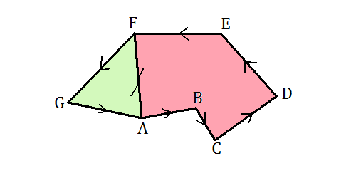
In the above, the quatnum phase of the pinkish region is given by Phase(ABCDEFA) while the quantum phase for the greenish region is given by Phase(AFGA). Adding these together gives the quantum phase for the region ABCDEFAFGA.

In the product ABCDEFAFGA, the internal sequence FAF is a complex multiple of the quantum state F. In the density operator language, SMS is how one computes the average of the operator M taken over the state S. In the usual language, this is written as = tr(SM) = tr(SMS). If the state M is Hermitian, this average is a real number and has no complex phase.

In our case, the state A is Hermitian, and therefore FAF is not just a complex multiple of F, but is instead a real multiple. We can therefore factor out this real multiple (which does not contribute to the phase), and replace FAF with F, and the product ABCDEFAFGA becomes ABCDEFGA. Thus we have shown the addition rule for the Berry phase of the Pauli algebra: Phase(ABCDEFA) + Phase(AFGA) = Phase(ABCDEFGA).

Berry Phase is Proportional to Area

We’ve shown (actually we would need more than this, but the other facts we will leave as an exercise for mathematicians with time on their hands) that Berry phase can be computed by breaking a large region up into smaller triangular regions. Since Berry phase is purely geometric, it cannot depend on the choice of coordinates and so cannot depend on where the triangle is located. Furthermore, we can make the triangles infinitesimal in size and Berry phase will have to be additive over these areas. It is easy to see (for a physicist who isn’t too interested in mathematical niceties) that Berry phase must be proportional to the area.

To compute the area of proportionality, we can consider an infinitesimal triangle made up of three directions near the z-axis, say u = (0,0,1), v = (0,d,1), and w = (d,0,1), where we keep values only to order d. The triangle is a right isoceles triangle with legs of length d. Its area is therefore . The three states U, V, W are given by:
U = (1+z)/2
V = (1+z+dy)/2
W = (1+z+dx)/2.

Computing the product of the quantum states, and leaving off factors of 2 which do not change he phase, we need
Phase(UVWU) = Phase( (1+z)(1+z+dy)(1+z+dx)(1+z) ).
To compute this, we need to remember that x, y, and z anticommute. The computation goes as follows. To 1st order in d we have:
Phase( (1+z)(1+z+dy)(1+z+dx)(1+z) )
= Phase ((1+z+dy+z+1+dzy)(1+z+dx+z+1+dxz) )
= Phase ((2+2z+dy+dzy)(2+2z+dx+dxz) )
= Phase ((4+4z+2dy+2dzy)+(4z+4+2dyz-2dy)+(2dx+2dzx)+(2dxz-2dx))
= Phase (8+8z+2dzy+2dyz+2dzx+2dxz)
= Phase (8+8z-2dyz+2dyz-2dxz+2dxz)
= Phase (8+8z) = Phase((1+z)/2) = 0

Ouch! We have to go to 2nd order in d! This is exactly what we expect since the area is 2nd order in d. The V and W states, to 2nd order in d are:
U = (1+z)/2
V = (1+(1-dd/2)z +dy)/2
W = (1+(1-dd/2)z+dx)/2.
Keeping only 2nd order terms in d, in the product we end up with (dd (-z + yx)). The operator z is spin in the z direction and the quantum states (1+z)/2 are eigenstates of this operator with eiegnvalue 1. So we can factor 1 into zz and rewrite the factors of order dd as:
dd (-z + yx) = dd (-z + zz yx) = dd (z)(-1 + zyx)
= dd(z)(-1 -xyz)
= dd (z) (-1 -i) .
The overall factor of z is absorbed into the (1+z)/2 factors as these are eigenstates of z. That is, (1+z)/2 z = (1+z)/2. And the factor (-1 – i) is a complex constant that can be factored out. This gives our calculational result as:
Phase (UVWU) =
= Phase ( (8+8z) – dd (1+z)(1+i)(1+z) )
= Phase ( (8+8z) – dd (2+2z)(1+i) )
= Phase ( (8+8z)(1 – dd (1+i)/4 ) )
= Phase ( (8+8z)( (1-dd/4) – i dd/4 ) )
The factor 8+8z is a real multiple of the primitive idempotent (1+z)/2 and so does not contribute to the phase which is
Phase ( (8+8z)( (1-dd/4) – i dd/4 ) )
= ArcTan ( (dd/4) / (1-dd/4) )
and to first order in dd, this is ArcTan(dd/4) = dd/4.

Since the triangle’s area was dd/2, we have that the proportionality ratio is 1/2, and the Berry phase associated with a spherical triangle (or any other spherical region) of area A is given by exp(i A/2). The minus sign comes from the ordering of the states; the area of the triangle is negative. To get a plus sign, reverse the order of the x and y contributions.

A previous post, Consistent Histories and Density Operator Formalism discussed the application of density matrices to the consistent histories interpretation of quantum mechanics with the practical appliction being Margaret Hawton’s photon position operator. The calculations there were similar to these in that probabilities were computed as multiples of the primitive idempotents. In both of these cases, the confused reader may insert a “trace” function. So the confused reader may write Phase(tr (ABCA) ) instead of Phase(ABCA), but I do not recommend this.

The reason for writing these sorts of things without the trace is several-fold. First, the trace is implied by the notation; one can’t take the phase of a matrix or interpret it as a probability without first doing something. But more importantly, when one is using this sort of QM to do non perturbational bound state problems, one needs to add up a lot of Feynman diagrams and the trace notation is inconvenient. And the machinery used here is more general than the trace. Berry phase applies to the representation of the Pauli algebra generated by any two anticommuting bilinears of the Dirac algebra. But in none of these cases is the product of the three bilinears equal to i. So the trace would give a result of zero on these sorts of calculations.

In the traditional method of working with Feynman diagrams, one transforms each diagram into a complex number and adds up these complex numbers to get the overall amplitude. However, in doing this, one finds that the Feynman diagrams that one has added together are each similar in that they share the same initial and final conditions. Putting that into density matrix formalism, the Feynman diagrams each share the same initial “A” and final “B” states, so the various diagrams will read as things like BMA, BM’A, BM”A, etc., where M, M’, and M” are various things that happen between the initial and final states.

So in the context of Feynman diagrams, it makes physical sense to do the trace function only after the diagrams have been added up. Mathematically it doesn’t matter, but in this point of view Feynman diagrams are not just complex numbers, they are complex multiples of a combination of initial and final states. In looking at bound states as collections of Feynman diagrams, one wishes to understand the algebra of Feynman diagrams, and this is much easier if one treats them as density matrices, and thinks of them as density matrices, rather than complex numbers.

Had fun learning about Berry phase using density matrices? Buy my book for this and many other cool things you can do in the density matrix formalism.